
For the original Knitr version HTML file, see here. It looks like the plugin of Pelican doesn't support Rmd perfectly.
1. Introduction
The sinking of Titanic in twentieth century is an sensational tragedy, in which 1502 out of 2224 passenger and crew members were killed. Kaggle provided this dataset to machine learning beginners to predict what sorts of people were more likely to survive given the information including sex, age, name, etc. Although the size of the dataset is small, it provides newbies a chance to accomplish most procedures in a data science project including data cleaning, feature engineering, model fitting, and tweaking to achieve higher scores.
1.1 Read the data
library(caret)

readData <- function(path.name, file.name, column.types, missing.types){
    read.csv(paste(path.name, file.name, sep=''), colClasses = column.types, na.strings = missing.types )
}
#Titanic.path <- './data/'
Titanic.path <- '/Users/caoxiang/Dropbox/Titanic/data/'
train.file.name <- 'train.csv'
test.file.name <- 'test.csv'
missing.types <- c('NA', '')
train.column.types <- c('integer',   # PassengerId
                        'factor',    # Survived
                        'factor',    # Pclass
                        'character', # Name
                        'factor',    # Sex
                        'numeric',   # Age
                        'integer',   # SibSp
                        'integer',   # Parch
                        'character', # Ticket
                        'numeric',   # Fare
                        'character', # Cabin
                        'factor'     # Embarked
)
test.column.types <- train.column.types[-2]

train <- readData(Titanic.path, train.file.name, train.column.types, missing.types)
test <- readData(Titanic.path, test.file.name, test.column.types, missing.types)
test$Survived <- NA # add Survived column to test dataset and fill it out with NA.

combi <- rbind(train, test) # combine training and test set for further manipulation
2. Exploratory Data Analysis
2.1 Check the structure of the dataset
str(train)
## 'data.frame':    891 obs. of  12 variables:
##  $ PassengerId: int  1 2 3 4 5 6 7 8 9 10 ...
##  $ Survived   : Factor w/ 2 levels "0","1": 1 2 2 2 1 1 1 1 2 2 ...
##  $ Pclass     : Factor w/ 3 levels "1","2","3": 3 1 3 1 3 3 1 3 3 2 ...
##  $ Name       : chr  "Braund, Mr. Owen Harris" "Cumings, Mrs. John Bradley (Florence Briggs Thayer)" "Heikkinen, Miss. Laina" "Futrelle, Mrs. Jacques Heath (Lily May Peel)" ...
##  $ Sex        : Factor w/ 2 levels "female","male": 2 1 1 1 2 2 2 2 1 1 ...
##  $ Age        : num  22 38 26 35 35 NA 54 2 27 14 ...
##  $ SibSp      : int  1 1 0 1 0 0 0 3 0 1 ...
##  $ Parch      : int  0 0 0 0 0 0 0 1 2 0 ...
##  $ Ticket     : chr  "A/5 21171" "PC 17599" "STON/O2. 3101282" "113803" ...
##  $ Fare       : num  7.25 71.28 7.92 53.1 8.05 ...
##  $ Cabin      : chr  NA "C85" NA "C123" ...
##  $ Embarked   : Factor w/ 3 levels "C","Q","S": 3 1 3 3 3 2 3 3 3 1 ...
summary(train)
##   PassengerId    Survived Pclass      Name               Sex
##  Min.   :  1.0   0:549    1:216   Length:891         female:314
##  1st Qu.:223.5   1:342    2:184   Class :character   male  :577
##  Median :446.0            3:491   Mode  :character
##  Mean   :446.0
##  3rd Qu.:668.5
##  Max.   :891.0
##
##       Age            SibSp           Parch           Ticket
##  Min.   : 0.42   Min.   :0.000   Min.   :0.0000   Length:891
##  1st Qu.:20.12   1st Qu.:0.000   1st Qu.:0.0000   Class :character
##  Median :28.00   Median :0.000   Median :0.0000   Mode  :character
##  Mean   :29.70   Mean   :0.523   Mean   :0.3816
##  3rd Qu.:38.00   3rd Qu.:1.000   3rd Qu.:0.0000
##  Max.   :80.00   Max.   :8.000   Max.   :6.0000
##  NA's   :177
##       Fare           Cabin           Embarked
##  Min.   :  0.00   Length:891         C   :168
##  1st Qu.:  7.91   Class :character   Q   : 77
##  Median : 14.45   Mode  :character   S   :644
##  Mean   : 32.20                      NA's:  2
##  3rd Qu.: 31.00
##  Max.   :512.33
##
2.2 Visualize the relationship between features and response
- Check the relation between
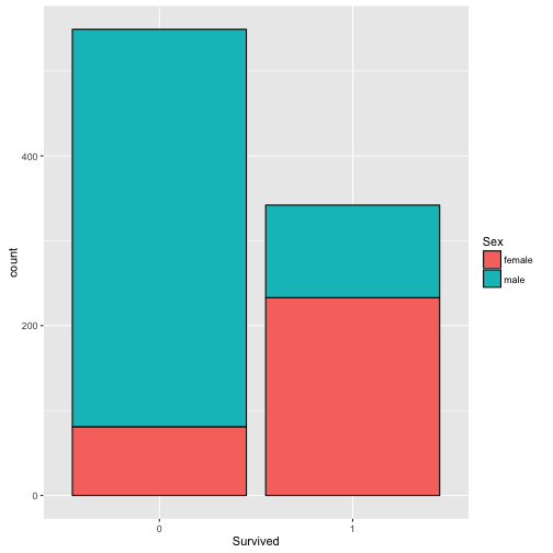
SexandSurvived
Consistent with our prior, the female is more likely to survive.
library(ggplot2)
p <- ggplot(train, aes(x=Survived, fill=Sex)) + geom_bar(color='black')
p
- Check the relation between
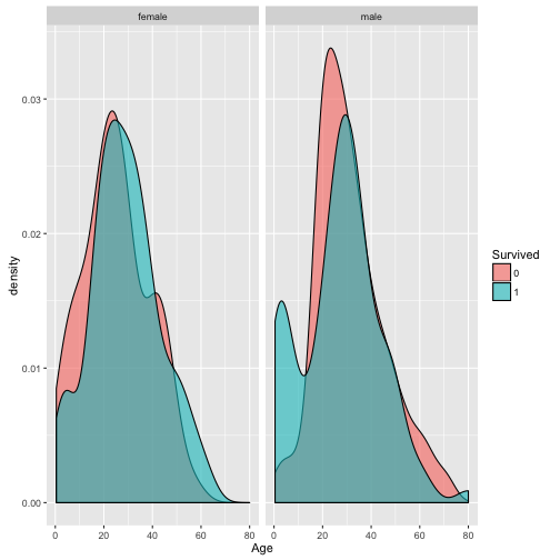
AgeandSurvive.
As there are many missing value in Age column, we omitted these rows before plotting. It looks like children are more likely to survive.
# show histogram
# p3 <- ggplot(train[!is.na(train$Age), ], aes(x=Age, fill=Survived)) + geom_histogram()
# show density plot
p2 <- ggplot(train[-which(is.na(train$Age)), ], aes(x=Age, fill=Survived)) + geom_density(alpha=0.6) +
    facet_grid(.~Sex)

p2
- Check the relation between
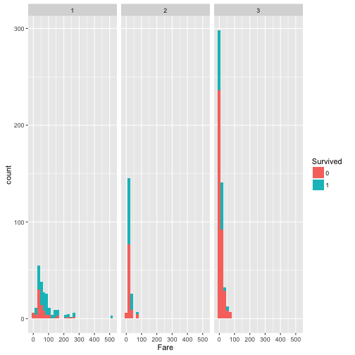
FareandSurvive.
Within the people who survived, higher percentage of them afforded high fare for the ticket, which indicates the high fare may correspond better cabins that are easy to escape from.
p3 <- ggplot(train, aes(x=Fare, fill=Survived)) + geom_histogram() +
    facet_grid(.~Pclass)
p3
prop.table(table(train$Survived, train$Pclass), margin = 2)
##
##             1         2         3
##   0 0.3703704 0.5271739 0.7576375
##   1 0.6296296 0.4728261 0.2423625
From the prop.table, compared to Pclass 2 and Pclass 3, higher percentage of passenger in Pclass 1 survived.
- Check the relation between
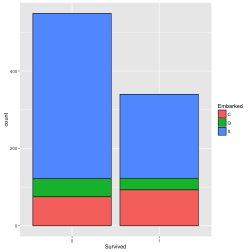
EmbarkedandSurvived.
No significant difference between port of embarkation.
p4 <- ggplot(train[!is.na(train$Embarked), ], aes(x=Survived, fill=Embarked)) + geom_bar(color='black')
p4
3. Data Clearing and Feature Engineering
3.1 Feature Engineering
Name. Extract thetitleandSurnamefromNameand create two new features.
title.extract <- function(x){
    strsplit(x, split = "[,.]")[[1]][2]
}
combi$Title <- sapply(combi$Name, FUN = title.extract)
combi$Title <- sub(" ", "", combi$Title) # delete the space in the Title

# combine the similiar into the same category
combi$Title[combi$PassengerId == 797] <- 'Mrs' # this passenger is a female doctor
combi$Title[combi$Title %in% c('Mlle', 'Mme')] <- 'Mlle'
combi$Title[combi$Title %in% c('Capt','Don','Major','Sir', 'Jonkheer')] <- 'Sir'
combi$Title[combi$Title %in% c('Dona', 'Lady', 'the Countess')] <- 'lady'
combi$Title <- as.factor(combi$Title)

combi$Surname <- sapply(combi$Name, FUN = function(x){strsplit(x, split="[,.]")[[1]][1]})
SibSpandParch. Create a new featureFamilySizewhich equalsSibSq + Parch +1
combi$FamilySize <- combi$SibSp + combi$Parch + 1
- Base on the two features
FamilySizeandSurname, we create a new featureFamilyIDin order to classify the passengers from the same family into groups. As there are many single passenger whose family is 1, we label these passengers whoseFamilySize <=2asSmall. Note there may be some records whoseFamilySizedoesn't equal the frequence ofFamilyID, it's obvious inconformity exists. So we labeled the records where frequence ofFamilyID <=2asSmallas well.
combi$FamilyID <- paste(as.character(combi$FamilySize), combi$Surname, sep = "")
combi$FamilyID[combi$FamilySize <= 2] <- "Small"
famIDs <- data.frame(table(combi$FamilyID))
famIDs <- famIDs[famIDs$Freq <= 2,]
# if famIDs frequency <=2, regard it as "Small" as well.
combi$FamilyID[combi$FamilyID %in% famIDs$Var1 ] <- "Small"
combi$FamilyID <- as.factor(combi$FamilyID)
- For
Cabin, we can extract the first letter ofCabinas a label. It's obviouse theCabinnumbers correspond different Passenger Class which is a crucial factor determining whether one could survive. However, since theCabinof most records are missing, although the importance of this variable seems to be significant in training, it doesn't increase the predicting score in my models.
# We write a function to extract the first letter of Cabin. A new factor 'N' is assigned to the missing values. Also, for the passengers with the same ticket number, the most frequent Cabin level besides 'N' is assigned to the rest passengers.

extractCabin <- function(combi){
    # extract the first letter of Cabin
    combi$Cabin <- sapply(combi$Cabin, FUN = function(x){strsplit(x, split='')[[1]][1]})
    combi$Cabin[is.na(combi$Cabin)] <- 'N'
    combi$Cabin <- as.factor(combi$Cabin)

    # set the same number tickets with the same Cabin label
    combi.ticket <- table(factor(combi$Ticket))
    combi.ticket.moreThanOne <- combi.ticket[combi.ticket>1]
    combi.temp <- combi[combi$Ticket %in% names(combi.ticket.moreThanOne), ]
    for(name in names(combi.ticket.moreThanOne)){
        row.sameTicket <- combi[combi$Ticket == name, ]
        Cabin_boolean <- row.sameTicket$Cabin %in% c('A','B','C','D','E','F','G')
        if(sum(Cabin_boolean) > 0){
            correctCabin <- names(sort(table(row.sameTicket$Cabin[Cabin_boolean]), decreasing=TRUE))[1]
            row.sameTicket$Cabin[row.sameTicket$Cabin == "N"] <- correctCabin
            # modify the Cabin of combi dataset
            combi$Cabin[row.sameTicket$PassengerId] <- row.sameTicket$Cabin
        }
    }
    combi$Cabin <- as.factor(combi$Cabin)
    return(combi)
}
combi <- extractCabin(combi)
- For
Ticket, we extracted the first alphabet character ofTicketto label the ticket.
extractTicket <- function(ticket){
    pattern <- c('\\/', '\\.', '\\s', '[[:digit:]]')
    for (p in pattern){
        # replace all chracter matches the pattern p with ""
        ticket <- gsub(p, "", ticket)
    }
    ticket <- substr(toupper(ticket), 1,1) # only extract the first alphabet character to label the ticket
    ticket[ticket==""] <- 'N'
    ticket <- as.factor(ticket)
}
combi$Ticket <- extractTicket(combi$Ticket)
3.2 Dealing with missing values
Fare. Replace the NA inFarewith the median ofFare.
combi$Fare[is.na(combi$Fare)] <- median(combi$Fare, na.rm = TRUE)
Embarked. Replase the NA inEmbarkedwith the most frequent labelS.
combi$Embarked[is.na(combi$Embarked)] <- "S"
Age. We fill out the NA inAgeby fitting a decision tree, which uses the features excludeSurvivedto predictAge. Here we just use the default parameters ofrpart, for more details, checkrpart.control.
library(rpart)
Agefit <- rpart(Age ~ Pclass + Sex + SibSp + Parch + Fare + Embarked + Title + FamilySize,
                data = combi[!is.na(combi$Age), ], method = "anova")
combi$Age[is.na(combi$Age)] <- predict(Agefit, combi[is.na(combi$Age), ])
4. Fitting Models
Write a function to extract features from dataset. As the dataset is small and many missing values in Cabin and Ticket, these two features actually don't increase the predicting score so I didn't included them in my models.
train <- combi[1:nrow(train), ]
test <- combi[nrow(train)+1 : nrow(test), ]

extractFeatures <- function(data){
    features <- c('Pclass',
                  'Sex',
                  'Age',
                  'SibSp',
                  'Parch',
                  'Fare',
                  #'Cabin',
                  'Embarked',
                  'Survived',
                  'Title',
                  'FamilySize',
                  'FamilyID'
                  #'Ticket'
    )
    fea <- data[ , features]
    return(fea)
}
4.1 Logistic regression (Ridge)
library(glmnet)

# create a sparse matrix of the dataset but column Survived. This is converting categorical variables into dummies variables.
x <- model.matrix(Survived~., data = extractFeatures(train))
y <- extractFeatures(train)$Survived
newx <- model.matrix(~., data = extractFeatures(test)[,-which(names(extractFeatures(test)) %in% 'Survived')])

set.seed(1)
fit_ridge <- cv.glmnet(x, y, alpha = 0, family = 'binomial', type.measure = 'deviance')
pred_ridge <- predict(fit_ridge, newx = newx, s = 'lambda.min', type='class')

submission <- data.frame(PassengerId = test$PassengerId, Survived = pred_ridge)
#write.csv(submission, file = "ridge.csv", row.names=FALSE)
The glmnet package can fit lasso, ridge and elasticnet. Here we just fit ridge which performs a little bit better than lasso in this dataset.
The submitted score is 0.80861.
Actually if you set set.seed(1), and use misclassification error as metric (set type.measure = 'class'), the submitted score can be as high as 0.82297. However, it seems the result of this metric isn't as stable as deviance.
4.2 Gradient boosting machine
Here we directly use Caret to fit the gradient boosting machine and tune parameters. Through Caret, there are four parameters can be tuned.
n.trees, the number of iterations (trees) in the model.interaction.depth, the numbers of splits it has to perform on a tree, so it equalsNumberOfLeaves + 1. Note: the interaction ininteraction.depthis defferent from the usual understanding which is the interaction of features, e.g. feature x has two levels A and B, feature y has two levels C and D, then the interaction of x and y has four levels.shrinkage, knows as learning rate, the empact of each tree on the final model. Lower learning rate requires more iterations.n.minobsinnode, minimum number of observations in the trees terminal nodes. The default value is 10.
For other parameters, like bag.fraction, cannot be tuned via Caret. You can write your function to tune it.
For the precedures of tuning GBM parameters in Python, see a blog here. The parameters of GBM in R is slightly different from the one in Python, but the experience of tuning is consistent.
library(caret)

fitControl <- trainControl(method = 'repeatedcv',
                           number = 3,
                           repeats = 3)
# for caret, there are only four tuning parameters below.

# tune n.trees
newGrid <- expand.grid(n.trees = c(50, 100, 200, 300),
                       interaction.depth = c(6),
                       shrinkage = 0.01,
                       n.minobsinnode = 10
                       )
fit_gbm <- train(Survived ~., data=extractFeatures(train),
                 method = 'gbm',
                 trControl = fitControl,
                 tuneGrid =  newGrid,
                 bag.fraction = 0.5,
                 verbose = FALSE)
fit_gbm$bestTune
##   n.trees interaction.depth shrinkage n.minobsinnode
## 3     200                 6      0.01             10
# tune interaction.depth
set.seed(1234)
newGrid <- expand.grid(n.trees = c(200),
                       interaction.depth = c(4:12),
                       shrinkage = 0.01,
                       n.minobsinnode = 10
                       )
fit_gbm <- train(Survived ~., data=extractFeatures(train),
                 method = 'gbm',
                 trControl = fitControl,
                 tuneGrid =  newGrid,
                 bag.fraction = 0.5,
                 verbose = FALSE)
fit_gbm$bestTune
##   n.trees interaction.depth shrinkage n.minobsinnode
## 7     200                10      0.01             10
# decrease learning rate
set.seed(1234)
newGrid <- expand.grid(n.trees = c(2000),
                       interaction.depth = c(10),
                       shrinkage = 0.001,
                       n.minobsinnode = 10
                       )
fit_gbm_LowerRate <- train(Survived ~., data=extractFeatures(train),
                 method = 'gbm',
                 trControl = fitControl,
                 tuneGrid =  newGrid,
                 bag.fraction = 0.5,
                 verbose = FALSE)
fit_gbm_LowerRate$results
##   n.trees interaction.depth shrinkage n.minobsinnode  Accuracy    Kappa
## 1    2000                10     0.001             10 0.8241676 0.618902
##   AccuracySD  KappaSD
## 1 0.03510324 0.072976
# predict
pred_gbm <- predict(fit_gbm_LowerRate, extractFeatures(test))
submission <- data.frame(PassengerId = test$PassengerId, Survived = pred_gbm)
#write.csv(submission, file = "gbm_ntree-2000_rate-0.001_inter-10.csv", row.names=FALSE)
The submitted score is 0.81340. As the size of data set is small, it seems the result of GBM isn't very stable for different random seed.
4.3 Random forest
This article is inspired by the excellent tutorial of Trevor Stephens, in which a conditional random forest is implemented to achieve the score of 0.81340. Here I just repeat this model.
library(party)
set.seed(1)
fit_crf <- cforest(Survived ~., data=extractFeatures(train), controls=cforest_unbiased(ntree=2000, mtry=3))
pred_crf <- predict(fit_crf, extractFeatures(test), OOB = TRUE, type="response")

submission <- data.frame(PassengerId = test$PassengerId, Survived = pred_crf)
#write.csv(submission, file = "crf_seed1.csv", row.names=FALSE)
The ntree is the number of trees in the random forest model, the mtry is the number of input variables randomly sampled as candidate at each node. The rule-of-thumb is sqrt(p) where p is the number of features, as we only included 10 features in our model, so we set mtry=3. For more details of conditional random forest, check help(ctree_contorl) in R. For the comparison between conditional inference trees and traditional decision trees, check the question in StackExchange.
The submitted score is 0.81340.
4.4. Ensemble
Ensemble is a effective way to combine the models to reduce the overall error rate. In one word, extracting the pattern discovered by each model and ensembling them could achieve a better score. Therefore, ensembling the uncorrelated results of models may do better since each model contain different patterns. For the detailed introduction of ensembling experiences, check this fantastic blog.
Here we just do the simple majority vote.
cat('Difference ratio between ridge and conditional random forest:', sum(pred_ridge!=pred_crf)/nrow(test))
## Difference ratio between ridge and conditional random forest: 0.06698565
cat('Difference ratio between ridge and conditional gbm:', sum(pred_ridge!=pred_gbm)/nrow(test))
## Difference ratio between ridge and conditional gbm: 0.0861244
cat('Difference ratio between conditional random forest and gbm:', sum(pred_crf!=pred_gbm)/nrow(test))
## Difference ratio between conditional random forest and gbm: 0.0430622
ensemble <- as.numeric(pred_ridge) + as.numeric(pred_gbm)-1 + as.numeric(pred_crf)-1
ensemble <- sapply(ensemble/3, round)

submission <- data.frame(PassengerId = test$PassengerId, Survived = ensemble)
#write.csv(submission, file = "ensemble_vote2.csv", row.names=FALSE)
The submitted score is 0.82297.
5. Summary
Logistic regression
- The
glmnetin R and logistic regression with l1 and l2 penalty in python sklearn are different. The cost function is different, sklearn regularize intercept while glmnet doesn't. See stackexchange as reference. - In
glmnet, before fitting the model, the data should be converted into sparse matrix(encode categorical variable into dummy variable). By defaultglmnetstandardize the input by default, including the dummy variables. According to the Tibshirani's article:-
The lasso method requires initial standardization of the regressors, so that the penalization scheme is fair to all regressors. For categorical regressors, one codes the regressor with dummy variables and then standardizes the dummy variables. As pointed out by a referee, however, the relative scaling between continuous and categorical variables in this scheme can be somewhat arbitrary.
-
- When tuning the regularization parameter $\lambda$ via
cv.glmnet,glmnetcalled one hundred values of lambda and choose the one which achieve lowest error. However for logistic regression in sklearn, a sequence of tuning parameterCneed be specified for tuning. As a result, logistic regression in sklearn can hardly performs as good asglmnet.
Gradient boosting
- Since the dataset is small, the performance of boosting machine isn't stable. This brings difficulty in tuning the parameters. Although some parameter combinations perform good through cross-validation on training set, they still overfit the test set.
Ensemble
- The ensemble method like stacking and blending may achieve better results, which could be the next step to tweak the model.
Comments
comments powered by Disqus