Data Wrangling: Quick Guide for dplyr, data.table and R build-in data.frame

The dplyr and data.table part are based on the courses Data Manipulation in R with dplyr and Data Manipulation in R, the data.table way on DataCamp. Hope the description along with the code in this guide help you understand the basic data wrangling in R clearly.

dplyr

Overview

Use tbl_df to convert data.frame into data frame table. tbl is a special type of data.frame.
glimpse (from tibble) display more info of the data table. It checks every column in the set, similar to R base function str.
Convert tbl back to data.frame. as.data.frame(iris)

data('iris')

# change names
names(iris) <- c('SL', 'SW', 'PL', 'PW', 'Species')

# covert the data.frame into tbl
library(dplyr)
iris <- tbl_df(iris)
iris # R only disply a portion of the tbl fits the console window

## # A tibble: 150 <U+00D7> 5
##       SL    SW    PL    PW Species
##    <dbl> <dbl> <dbl> <dbl>  <fctr>
## 1    5.1   3.5   1.4   0.2  setosa
## 2    4.9   3.0   1.4   0.2  setosa
## 3    4.7   3.2   1.3   0.2  setosa
## 4    4.6   3.1   1.5   0.2  setosa
## 5    5.0   3.6   1.4   0.2  setosa
## 6    5.4   3.9   1.7   0.4  setosa
## 7    4.6   3.4   1.4   0.3  setosa
## 8    5.0   3.4   1.5   0.2  setosa
## 9    4.4   2.9   1.4   0.2  setosa
## 10   4.9   3.1   1.5   0.1  setosa
## # ... with 140 more rows

# change column names
names(iris) <- c('SL', 'SW', 'PL', 'PW', 'Species')

# change the level name of factor
new_level <- c('setasa'='set', 'versicolor'='ver', 'virginica'='vir')
iris$new_Species <- as.factor(new_level[iris$Species])

# check more info of data table
glimpse(iris)

## Observations: 150
## Variables: 6
## $ SL          <dbl> 5.1, 4.9, 4.7, 4.6, 5.0, 5.4, 4.6, 5.0, 4.4, 4.9, ...
## $ SW          <dbl> 3.5, 3.0, 3.2, 3.1, 3.6, 3.9, 3.4, 3.4, 2.9, 3.1, ...
## $ PL          <dbl> 1.4, 1.4, 1.3, 1.5, 1.4, 1.7, 1.4, 1.5, 1.4, 1.5, ...
## $ PW          <dbl> 0.2, 0.2, 0.2, 0.2, 0.2, 0.4, 0.3, 0.2, 0.2, 0.1, ...
## $ Species     <fctr> setosa, setosa, setosa, setosa, setosa, setosa, s...
## $ new_Species <fctr> set, set, set, set, set, set, set, set, set, set,...

Five verbs for data manipulation. select, filter, arrange, mutate, summarize.

`select()`

Select(Remove) the columns by name and return a table which contains the selected columns. The original table is not modified. If you want to use the returned table later, save it into a new object. new_table <- select(iris, var1, var2).

The grammer is select(data, var1, var2). We can put variable names into a string c(var1, var2) also.
Use colon : to select a range of columns. Use - to drop columns. select(data, var1:var4, -var2).
select also works with column index. select(data, 1:4, -2)
Helper function for selection, check select_helpers.
- starts_with("X"): every name that starts with "X",
- ends_with("X"): every name that ends with "X",
- contains("X"): every name that contains "X",
- matches("X"): every name that matches "X", where "X" can be a regular expression,
- num_range("x", 1:5): the variables named x01, x02, x03, x04 and x05,
- one_of(x): every name that appears in x, which should be a character vector.
select_ accepts string(only) as paramters which used often when programming with select.

select(iris, SL, Species) # select two columns

## # A tibble: 150 <U+00D7> 2
##       SL Species
##    <dbl>  <fctr>
## 1    5.1  setosa
## 2    4.9  setosa
## 3    4.7  setosa
## 4    4.6  setosa
## 5    5.0  setosa
## 6    5.4  setosa
## 7    4.6  setosa
## 8    5.0  setosa
## 9    4.4  setosa
## 10   4.9  setosa
## # ... with 140 more rows

# select(iris, SL:Species, -SW) # select columns between SL and Species except SW
# select(iris, c(1:2, 4:5))
# select(iris, 1:3, -2) # select columns between index 1 and 3 except 2
# select(iris, starts_with('S'), ends_with('L')) # for more than one helper function, the relation is `OR`

`mutate()`

Use the data to build new columns and update the original data set.
The new created column can be referred in later expression.

iris_2 <- mutate(iris, area_S = SL*SW, area_S2 = area_S^2)
head(iris_2)

## # A tibble: 6 <U+00D7> 8
##      SL    SW    PL    PW Species new_Species area_S  area_S2
##   <dbl> <dbl> <dbl> <dbl>  <fctr>      <fctr>  <dbl>    <dbl>
## 1   5.1   3.5   1.4   0.2  setosa         set  17.85 318.6225
## 2   4.9   3.0   1.4   0.2  setosa         set  14.70 216.0900
## 3   4.7   3.2   1.3   0.2  setosa         set  15.04 226.2016
## 4   4.6   3.1   1.5   0.2  setosa         set  14.26 203.3476
## 5   5.0   3.6   1.4   0.2  setosa         set  18.00 324.0000
## 6   5.4   3.9   1.7   0.4  setosa         set  21.06 443.5236

`filter()`

Remove the rows.
Use filter together with relational operators. Check Comparison. <, >, <=, >=, ==, !=, %in%.
For more than one conditions, use boolean operators &, |, !.
filter_ accepts string as parameters as well.

filter(iris, SL == 5.1 & SW >=3.5)

## # A tibble: 6 <U+00D7> 6
##      SL    SW    PL    PW Species new_Species
##   <dbl> <dbl> <dbl> <dbl>  <fctr>      <fctr>
## 1   5.1   3.5   1.4   0.2  setosa         set
## 2   5.1   3.5   1.4   0.3  setosa         set
## 3   5.1   3.8   1.5   0.3  setosa         set
## 4   5.1   3.7   1.5   0.4  setosa         set
## 5   5.1   3.8   1.9   0.4  setosa         set
## 6   5.1   3.8   1.6   0.2  setosa         set

`arrange()`

Reorder the rows in a data set
Use desc() to arrange in descending order, defaul is ascending.
Support arrange by several variables using comma ,.

# rearrange the table by SL and SW in ascending order
arrange(iris, SL, SW)

## # A tibble: 150 <U+00D7> 6
##       SL    SW    PL    PW Species new_Species
##    <dbl> <dbl> <dbl> <dbl>  <fctr>      <fctr>
## 1    4.3   3.0   1.1   0.1  setosa         set
## 2    4.4   2.9   1.4   0.2  setosa         set
## 3    4.4   3.0   1.3   0.2  setosa         set
## 4    4.4   3.2   1.3   0.2  setosa         set
## 5    4.5   2.3   1.3   0.3  setosa         set
## 6    4.6   3.1   1.5   0.2  setosa         set
## 7    4.6   3.2   1.4   0.2  setosa         set
## 8    4.6   3.4   1.4   0.3  setosa         set
## 9    4.6   3.6   1.0   0.2  setosa         set
## 10   4.7   3.2   1.3   0.2  setosa         set
## # ... with 140 more rows

# in descending order
# arrange(iris, SL, desc(SW))

# arrange by sum of SL and SW
# arrange(iris, SL+SW)

`summarise()`

Calculate summary statistics. summarise(tbl, sum=sum(A), avg=mean(B), var=var(B))
You can use any function in summarise as long as the function can take a vector of data and return a single number. min, max, mean, median, quantile(x, p) -p is the quantile of vector x, sd, var, IQR -Inter Quartile Range of vector x, diff(range(x)) -total range of vector x.
dplyr aggrgate function.
- first(x), last(x), nth(x, n) -the nth element of vector x.
- n() -the number of rows in the data.frame or group of observations that summarise() describes.
- n_distinct(x) -the number of unique values in vector x.

summarise(iris, mean_SL=mean(SL), nth_PW=nth(PW, 10), distinct_Species=n_distinct(Species), N=n())

## # A tibble: 1 <U+00D7> 4
##    mean_SL nth_PW distinct_Species     N
##      <dbl>  <dbl>            <int> <int>
## 1 5.843333    0.1                3   150

pipe operator `%>%`

From magrittr package. Effecient, readable, save space in memory. We don't need use nested loop. object %>% function( , arg2, arg3), object is passed as the first argument in the function, and it is written as object %>% function(arg2, arg3)

# use pipe operator to mutate, then filter
iris %>%
  mutate(area_S = SL*SW) %>%
  filter(Species == 'setosa' & SW > 3) %>%
  summarise(avg = mean(area_S))

## # A tibble: 1 <U+00D7> 1
##        avg
##      <dbl>
## 1 17.98048

`group_by`

Takes an existing tbl and converts it into grouped tbl where operations are performed by group. Its influence becomes clear when calling summarise() on a grouped dataset: summarising statistics are calculated for the different groups separately.

iris %>%
  group_by(Species) %>%
  summarise(avg_SL = mean(SL, na.rm=TRUE), avg_SW = mean(SW)) %>%
  arrange(avg_SW)

## # A tibble: 3 <U+00D7> 3
##      Species avg_SL avg_SW
##       <fctr>  <dbl>  <dbl>
## 1 versicolor  5.936  2.770
## 2  virginica  6.588  2.974
## 3     setosa  5.006  3.428

# or we can use:
iris %>%
  group_by(Species) %>%
  summarise(avg_SL = mean(SL, na.rm=TRUE), avg_SW = mean(SW)) %>%
  mutate(rank = rank(avg_SL)) %>%
  arrange(rank)

## # A tibble: 3 <U+00D7> 4
##      Species avg_SL avg_SW  rank
##       <fctr>  <dbl>  <dbl> <dbl>
## 1     setosa  5.006  3.428     1
## 2 versicolor  5.936  2.770     2
## 3  virginica  6.588  2.974     3

dplyr also works with other data set types like data.table, data.frame.

data.table

Overview

Think data.frame as a set of columns. data.table inherits from data.frame, but reduces programming time and computing time. data.table is data.frame, accepted as a data.frame by other pacakges. For the packages don't know data.table, DT[...] is redirected to data.frame methods for square bracket [...].
General form: DT[i, j, by], i corresponds WHERE in SQL and j corresponds SELECT in SQL. It stands for "Take DT, subset rows using i, then calculate j grouped by by".

Select rows by argument `i`

Comma , can be ignored. For data.table, iris[1:3] equals to iris[1:3, ]. But for data.frame, iris[1:3] returns error if you forget comma.
.N, a special symbol which contains the number of rows when used inside square brackets.

data('iris')

# change names
names(iris) <- c('SL', 'SW', 'PL', 'PW', 'Species')

# covert data.frame to data.table
library(data.table)
iris <- data.table(iris)

# select rows
iris[1:3]  # iris[1:3,] returns the same table.

##     SL  SW  PL  PW Species
## 1: 5.1 3.5 1.4 0.2  setosa
## 2: 4.9 3.0 1.4 0.2  setosa
## 3: 4.7 3.2 1.3 0.2  setosa

# select the first and second last row.
iris[c(1, .N-1)]

##     SL  SW  PL  PW   Species
## 1: 5.1 3.5 1.4 0.2    setosa
## 2: 6.2 3.4 5.4 2.3 virginica

Select columns by argument `j`

Select columns by j. Put j into .(), an alias to list() in data.tables and they mean the same. iris[, .(SL, SW)]. Note DT[, .(B)] returns a data.table, while DT[, B] returns a vector, so is DT[['B']], note column name contained in quotation. And DT[, c(B,C)] returns a vector combined with B and C.
Compute on columns. iris[, .(mean_SL=mean(SL), mean_SW=mean(SW)].
The generated multiple columns all return the same length. The length of short item get recycled to match the length of large columns. iris[, .(SL, mean_SL=mean(SL)). For all rows, they have the same mean_SL.
Throw anything into j. iris[, plot(SL, SW)].
Subsetting data.tables. DT[1:3, 2:4, with=False]. Check the argument with. The argument is named with because it determines whether the column index should be evaluated within the frame of the data.table, as it would be when using, e.g., base R's with() and within(). When with=FALSE j is a character vector of column names or a numeric vector of column positions to select.

# select three columns
iris[1:3, .(SL, PL, SW)]

##     SL  PL  SW
## 1: 5.1 1.4 3.5
## 2: 4.9 1.4 3.0
## 3: 4.7 1.3 3.2

# select two columns together with a generated column
iris[, .(SL, SW, area_S = SL*SW)]

##       SL  SW area_S
##   1: 5.1 3.5  17.85
##   2: 4.9 3.0  14.70
##   3: 4.7 3.2  15.04
##   4: 4.6 3.1  14.26
##   5: 5.0 3.6  18.00
##  ---               
## 146: 6.7 3.0  20.10
## 147: 6.3 2.5  15.75
## 148: 6.5 3.0  19.50
## 149: 6.2 3.4  21.08
## 150: 5.9 3.0  17.70

# throw anything into `j`
iris[, {print(head(SW))
        hist(SW)
        NULL}] # return NULL

## [1] 3.5 3.0 3.2 3.1 3.6 3.9

plot of chunk unnamed-chunk-10

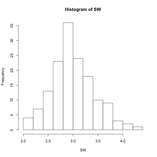
## NULL

# select column using index. Set with=FALSE.
iris[1:3, 2:4, with=FALSE] # the same as R base. If iris is data.frame. iris[1:3,2:4] returns the same

##     SW  PL  PW
## 1: 3.5 1.4 0.2
## 2: 3.0 1.4 0.2
## 3: 3.2 1.3 0.2

# also we can use column name
iris[1:3, SW:PW, with=FALSE]

##     SW  PL  PW
## 1: 3.5 1.4 0.2
## 2: 3.0 1.4 0.2
## 3: 3.2 1.3 0.2

Doing `j` by group

by can have more than one values. by = .(A, B)
We can call functions in by
Shortcut: if there is only one item in j or by, you can drop the .() notation.

iris[, .(mean_SL = mean(SL)), by=.(Species)]

##       Species mean_SL
## 1:     setosa   5.006
## 2: versicolor   5.936
## 3:  virginica   6.588

# call function in `by`, and grouping only on a subset
iris[1:100, .(mean_SL = mean(SL)), by=.(substr(Species, 1, 1))] # group by the 1st character of Species

##    substr mean_SL
## 1:      s   5.006
## 2:      v   5.936

# count the number of rows by group
iris[, .(Count = .N), by=.(not_setosa <- Species != 'setosa')]

##    not_setosa Count
## 1:      FALSE    50
## 2:       TRUE   100

# select the last two rows of SL by group 
iris[, .(last_two_SL = tail(SL, 2)), by=.(Species)]

##       Species last_two_SL
## 1:     setosa         5.3
## 2:     setosa         5.0
## 3: versicolor         5.1
## 4: versicolor         5.7
## 5:  virginica         6.2
## 6:  virginica         5.9

Chaining

Chain two [], [] together.

# select the last two rows of SL by group
iris[, .(SL), by=.(Species)][, .(last_two_SL = tail(SL,2)), by=.(Species)]

##       Species last_two_SL
## 1:     setosa         5.3
## 2:     setosa         5.0
## 3: versicolor         5.1
## 4: versicolor         5.7
## 5:  virginica         6.2
## 6:  virginica         5.9

# order by selected column
iris[, .(last_two_SL = tail(SL, 2)), by=.(Species)][order(last_two_SL, decreasing = TRUE)]

##       Species last_two_SL
## 1:  virginica         6.2
## 2:  virginica         5.9
## 3: versicolor         5.7
## 4:     setosa         5.3
## 5: versicolor         5.1
## 6:     setosa         5.0

Subset of data

A special built-in variable .SD, refers to the subset of the data table for each unique value of the by argument.
.SDcols specifies the columns of DT that are included in .SD. Use .SDcols if you want to perform a particular operation on a subset of the columns.

# use lapply to compute the mean of each columns
iris[, lapply(.SD, mean), by = .(Species)]

##       Species    SL    SW    PL    PW
## 1:     setosa 5.006 3.428 1.462 0.246
## 2: versicolor 5.936 2.770 4.260 1.326
## 3:  virginica 6.588 2.974 5.552 2.026

# use .SDcols to specify the columns(2nd to 4th) selected for each group.
iris[, lapply(.SD, mean), .SDcols = c(2:4), by = .(Species)]

##       Species    SW    PL    PW
## 1:     setosa 3.428 1.462 0.246
## 2: versicolor 2.770 4.260 1.326
## 3:  virginica 2.974 5.552 2.026

# we can also set the value of .SDcols as column names. e.g. .SDcols = c('SL', 'SW')
iris[, lapply(.SD, mean), .SDcols = c('SL', 'SW'), by = .(Species)] # note add quotation ""

##       Species    SL    SW
## 1:     setosa 5.006 3.428
## 2: versicolor 5.936 2.770
## 3:  virginica 6.588 2.974

Using `:=` in `j`

Updates the data table by reference.
Different from selecting by i and j, this is updating data table, and the new data table isn't printed.
Remove columns using := NULL. Remove the columns instantly no matter how large the data is in RAM. The columns can be indicated by both name or column index number.
Functional :=. DT[,:=(y=6:10, )
:= combined with i and by. Note if i is set a value, then only those rows are used to compute in the := by groups. It doesn't mean select i rows in the updated data table. See example in code chunk below.

# reverse a column, create a new column
iris[, c('rev_SL', 'area_S') := .(rev(SL), SL*SW)]

# remove a column. If only one column, there is shortcut: iris[, area_S := NULL]
iris[, c('rev_SL', 'area_S') := NULL] 

# if the columns need be deleted is a vector, we need add bracket to stop the variable being a symbol. 
# Then data.table knows to look up the value of the variable.
# Also, you can paste 

# MyCols <- c('rev_SL', 'area_S')
# iris[, (MyCols) := NULL]

# Functional :=
iris[, `:=`(x = 6:10, # space of comment for each variable, make it easy to read 
            z = 1)]

# := combined with i and by
# only the 1st 100 rows are selected to compute mean of SL by Species. The `mean_SL` in rows later than 100 are NA
iris[1:100, mean_SL:=mean(SL), by=.(Species)] 
iris[c(1:3, 101:103)]

##     SL  SW  PL  PW   Species x z mean_SL
## 1: 5.1 3.5 1.4 0.2    setosa 6 1   5.006
## 2: 4.9 3.0 1.4 0.2    setosa 7 1   5.006
## 3: 4.7 3.2 1.3 0.2    setosa 8 1   5.006
## 4: 6.3 3.3 6.0 2.5 virginica 6 1      NA
## 5: 5.8 2.7 5.1 1.9 virginica 7 1      NA
## 6: 7.1 3.0 5.9 2.1 virginica 8 1      NA

# an error for deleting columns
iris[, c('x') := NULL] # not error is given if i is specified.
iris[, 6 := NULL] # remove column by number also works.

Use `set()`

Assignment by reference, used to repeatedly update a data.table by reference. You can think of the set() as loopable, low overhead version of the := operator, except that set() cannot be used for grouping operations. set(DT, index, column, value)

# randomly set three items in 6th column to be NA 
temp <- iris[1:6]
for(i in 6:6) set(temp, sample.int(nrow(temp), 3), i, NA)
temp

##     SL  SW  PL  PW Species mean_SL
## 1: 5.1 3.5 1.4 0.2  setosa      NA
## 2: 4.9 3.0 1.4 0.2  setosa   5.006
## 3: 4.7 3.2 1.3 0.2  setosa      NA
## 4: 4.6 3.1 1.5 0.2  setosa   5.006
## 5: 5.0 3.6 1.4 0.2  setosa   5.006
## 6: 5.4 3.9 1.7 0.4  setosa      NA

Use `setnames()`, `setcolorder`

Use setnames() to set or change column names; use setcolorder() to reorder the columns.

setnames(temp, names(temp), paste0(names(temp), '_new'))
temp[1]

##    SL_new SW_new PL_new PW_new Species_new mean_SL_new
## 1:    5.1    3.5    1.4    0.2      setosa          NA

Indexing

Automatic indexing. Data table don't actually vector scan. They create an index automatically on SL the first time you use column SL. So second time it's much faster as the index alread exists. In data base, you need create the index by hand, while in data.table it's done automatically.

head(iris[SL >0 & SL <10 & !Species %in% c('setosa')])

##     SL  SW  PL  PW    Species mean_SL
## 1: 7.0 3.2 4.7 1.4 versicolor   5.936
## 2: 6.4 3.2 4.5 1.5 versicolor   5.936
## 3: 6.9 3.1 4.9 1.5 versicolor   5.936
## 4: 5.5 2.3 4.0 1.3 versicolor   5.936
## 5: 6.5 2.8 4.6 1.5 versicolor   5.936
## 6: 5.7 2.8 4.5 1.3 versicolor   5.936

iris[SL >1 & SL <11] # second time much faster.

##       SL  SW  PL  PW   Species mean_SL
##   1: 5.1 3.5 1.4 0.2    setosa   5.006
##   2: 4.9 3.0 1.4 0.2    setosa   5.006
##   3: 4.7 3.2 1.3 0.2    setosa   5.006
##   4: 4.6 3.1 1.5 0.2    setosa   5.006
##   5: 5.0 3.6 1.4 0.2    setosa   5.006
##  ---                                  
## 146: 6.7 3.0 5.2 2.3 virginica      NA
## 147: 6.3 2.5 5.0 1.9 virginica      NA
## 148: 6.5 3.0 5.2 2.0 virginica      NA
## 149: 6.2 3.4 5.4 2.3 virginica      NA
## 150: 5.9 3.0 5.1 1.8 virginica      NA

# remove the `_new` suffix
setnames(temp, names(temp), gsub('\\_new$', '', names(temp))) # `^` means begin with, `$` means end with.
temp[1]

##     SL  SW  PL  PW Species mean_SL
## 1: 5.1 3.5 1.4 0.2  setosa      NA

# remove the columns end with `_SL`
temp[, names(temp)[grepl('\\_SL$', names(temp))] := NULL]
temp[1]

##     SL  SW  PL  PW Species
## 1: 5.1 3.5 1.4 0.2  setosa

Keys

Set keys on columns, setkey(DT, A), then use DT['b'] to filter the rows where A == 'b'. (effectively filter). To data.frame, it turns to error.
Two-column key setkey(DT, A, B). The second column is sorted within each group of the first column
by = .EACHI, allows to group by each subset of knows groups in i. A key needs to be set prior to use by = .EACHI.

setkey(iris, Species)
head(iris['setosa'])

##     SL  SW  PL  PW Species mean_SL
## 1: 5.1 3.5 1.4 0.2  setosa   5.006
## 2: 4.9 3.0 1.4 0.2  setosa   5.006
## 3: 4.7 3.2 1.3 0.2  setosa   5.006
## 4: 4.6 3.1 1.5 0.2  setosa   5.006
## 5: 5.0 3.6 1.4 0.2  setosa   5.006
## 6: 5.4 3.9 1.7 0.4  setosa   5.006

iris['setosa', mult = 'first'] # 'last' returns the last row

##     SL  SW  PL  PW Species mean_SL
## 1: 5.1 3.5 1.4 0.2  setosa   5.006

# nomatch
iris['otherSpecies', nomatch = NA] # default

##    SL SW PL PW      Species mean_SL
## 1: NA NA NA NA otherSpecies      NA

iris['otherSpecies', nomatch = 0]

## Empty data.table (0 rows) of 6 cols: SL,SW,PL,PW,Species,mean_SL

# set two-column key. The second column is sorted within each group of the first column
setkey(iris, Species, SW)
head(iris)

##     SL  SW  PL  PW Species mean_SL
## 1: 4.5 2.3 1.3 0.3  setosa   5.006
## 2: 4.4 2.9 1.4 0.2  setosa   5.006
## 3: 4.9 3.0 1.4 0.2  setosa   5.006
## 4: 4.8 3.0 1.4 0.1  setosa   5.006
## 5: 4.3 3.0 1.1 0.1  setosa   5.006
## 6: 5.0 3.0 1.6 0.2  setosa   5.006

iris[.('setosa', 3)]

##     SL SW  PL  PW Species mean_SL
## 1: 4.9  3 1.4 0.2  setosa   5.006
## 2: 4.8  3 1.4 0.1  setosa   5.006
## 3: 4.3  3 1.1 0.1  setosa   5.006
## 4: 5.0  3 1.6 0.2  setosa   5.006
## 5: 4.4  3 1.3 0.2  setosa   5.006
## 6: 4.8  3 1.4 0.3  setosa   5.006

# first and last row of the `setosa` group
iris[c('setosa'), .SD[c(1, .N)], by=.EACHI]

##    Species  SL  SW  PL  PW mean_SL
## 1:  setosa 4.5 2.3 1.3 0.3   5.006
## 2:  setosa 5.7 4.4 1.5 0.4   5.006

Rolling joins

The value we are looking for falls in a gap in the ordered series in a key. See more details here. It's often used in time series data.

DT <- data.table(A= letters[1:3], B=1:6, C=6:1)
setkey(DT, A, B)
DT

##    A B C
## 1: a 1 6
## 2: a 4 3
## 3: b 2 5
## 4: b 5 2
## 5: c 3 4
## 6: c 6 1

DT[.('b', 4)] # C is NA

##    A B  C
## 1: b 4 NA

DT[.('b', 4), roll = TRUE] # C is 5

##    A B C
## 1: b 4 5

DT[.('b', 4), roll = 'nearest'] # C is 2

##    A B C
## 1: b 4 2

DT[.('b', 4), roll = +Inf]

##    A B C
## 1: b 4 5

DT[.('b', 4), roll = -Inf]

##    A B C
## 1: b 4 2

DT[.('b', 4), roll = TRUE, rollends = FALSE]

##    A B C
## 1: b 4 5

R build-in data.frame

Overview of data.frame

data('iris')
# change names
names(iris) <- c('SL', 'SW', 'PL', 'PW', 'Species')
str(iris)

## 'data.frame':    150 obs. of  5 variables:
##  $ SL     : num  5.1 4.9 4.7 4.6 5 5.4 4.6 5 4.4 4.9 ...
##  $ SW     : num  3.5 3 3.2 3.1 3.6 3.9 3.4 3.4 2.9 3.1 ...
##  $ PL     : num  1.4 1.4 1.3 1.5 1.4 1.7 1.4 1.5 1.4 1.5 ...
##  $ PW     : num  0.2 0.2 0.2 0.2 0.2 0.4 0.3 0.2 0.2 0.1 ...
##  $ Species: Factor w/ 3 levels "setosa","versicolor",..: 1 1 1 1 1 1 1 1 1 1 ...

Subset a data.frame

Dollar sign $. iris$SL returns a vector, so is iris[, 'SL'].
iris['SL'] returns one column as data.frame

# select two columns and return data.frame
iris[c('SL', 'SW')][1,]

##    SL  SW
## 1 5.1 3.5

# use subset()
subset(iris, select = c('SL', 'PL'))[1,]

##    SL  PL
## 1 5.1 1.4

# use index along with relational operators
iris[iris$SL > 7 & !is.na(iris$Species), 1:3][1, ]

##      SL SW  PL
## 103 7.1  3 5.9

# use `-` to delete columns by column index. Both with or without a comma work 
iris[-5][1, ]

##    SL  SW  PL  PW
## 1 5.1 3.5 1.4 0.2

iris[, -5][1, ]

##    SL  SW  PL  PW
## 1 5.1 3.5 1.4 0.2

# other expressions to delete columns
# delCols <- 'Species'
# iris[! names(iris) %in% delCols][1, ]
# iris[, ! names(iris) %in% delCols][1, ]
# iris[ -which(names(iris) %in% delCols)][1, ]
# iris[, -which(names(iris) %in% delCols)][1, ]

Add a column

iris$is_setosa <- iris$Species == 'setosa'
iris[1, ]

##    SL  SW  PL  PW Species is_setosa
## 1 5.1 3.5 1.4 0.2  setosa      TRUE

Combine R object by rows or columns.

# combine by columns. Note the short item is recycled to match the length of large columns.
cbind(iris, z=1)[1, ]

##    SL  SW  PL  PW Species is_setosa z
## 1 5.1 3.5 1.4 0.2  setosa      TRUE 1

Sort data.frame by columns

Use function order. The return of order() are the indices of the ordered vector.

# an example for order. the return of order() are the indices of the ordered vector
# as below, in order(s), 1 is the index of first number(1) of ordered vector(1 2 4 5 7) in original vector. 
# 5 is the index of second number(2) of ordered vector(1 2 4 5 7) in original vector, which is 5th.
s <- c(1,5,7,4,2)
sort(s)     # [1] 1 2 4 5 7

## [1] 1 2 4 5 7

order(s)    # [1] 1 5 4 2 3

## [1] 1 5 4 2 3

s[order(s)] # [1] 1 5 4 2 3

## [1] 1 2 4 5 7

# sort data.frame by multiple columns
head(iris[order(iris$SL, -iris$SW), ])

##     SL  SW  PL  PW Species is_setosa
## 14 4.3 3.0 1.1 0.1  setosa      TRUE
## 43 4.4 3.2 1.3 0.2  setosa      TRUE
## 39 4.4 3.0 1.3 0.2  setosa      TRUE
## 9  4.4 2.9 1.4 0.2  setosa      TRUE
## 42 4.5 2.3 1.3 0.3  setosa      TRUE
## 23 4.6 3.6 1.0 0.2  setosa      TRUE

dplyr

Overview

select()

mutate()

filter()

arrange()

summarise()

pipe operator %>%

group_by

data.table

Overview

Select rows by argument i

Select columns by argument j

Doing j by group

Chaining

Subset of data

Using := in j

Use set()

Use setnames(), setcolorder

Indexing

Keys

Rolling joins

R build-in data.frame

Overview of data.frame

Subset a data.frame

Add a column

Combine R object by rows or columns.

Sort data.frame by columns

Comments

`select()`

`mutate()`

`filter()`

`arrange()`

`summarise()`

pipe operator `%>%`

`group_by`

Select rows by argument `i`

Select columns by argument `j`

Doing `j` by group

Using `:=` in `j`

Use `set()`

Use `setnames()`, `setcolorder`